Team Members
Bhon Bunnag, Sean McGovern, Ying Fang, Mengdi Li, Jidapa Thadajarassiri
Motivation
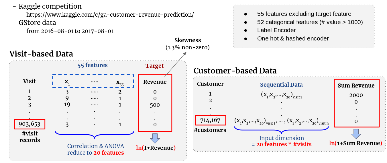
The ‘Google Analytics Customer Revenue Prediction’ is a Kaggle competition to predict the revenue generated per customer from data of the Google Merchandise Store (GStore). The data presents us with a skewed target variable, where only a small number of customer visits generate non-zero revenue. Some customers may also visit the GStore multiple times, which produces sequential data. State of the art algorithms such as linear regression and regression trees are insufficient for predicting skewed and sequential data. As such, we propose a joint classification-regression technique, which is more robust against skewed data. Recurrent Neural Networks (RNN) will be integrated into the proposed system to handle sequential data. Business owners will obviously find this joint model useful to analyze customer generated revenue. Furthermore, this model can be generalized to be used for any sequential data with skewed target variable.
Problem Statement and Challenge
We would like to implement machine learning systems that accurately predicts customer generated revenue. The dataset being used is very skewed. The dataset also contains recursive data instances.
Data
The dataset is provided by Kaggle competition. There are 903,653 visiting records with 55 features of visiting information, such as visitDate, visitorID and visitNumber. The records are from 2016-08-01 to 2017-08-01. A visitor corresponds to one or many visiting records, which produces sequential data. Among the useful 33 features, besides the 4 ID and 2 datetime features, there are 4 numerical features and 23 categorical features. The target variable is “totals.transactionRevenue”. It is noticeable that only 11,515 visiting records (<1.3%) of the dataset contains non-zero value.
Visit-based Model
State of the Art
Linear Regression is a classic state of the art algorithm for predicting real numerical target variables. However, linear regression will produce high bias, and not suitable for the dataset if the ground truth relationship in the dataset is non-linear. Polynomial regression will solve these issues, but may lead to overfitting. Decision Tree is also another usable state of the art algorithm for this task. Given that both categorical and numerical features are present in the dataset, the decision tree may be more suitable than Linear/Polynomial regression. Additionally, this algorithm also performs feature selection automatically.
Linear Regression Code in Python
from sklearn.metrics import mean_squared_error
from sklearn.linear_model import LinearRegression

train_mse = []
train_rmse = []
val_mse = []
val_rmse = []

for i in range(fold):

	print('\n\nfold:', i)
	val = processed_train_df[processed_train_df['fullVisitorId'].isin(id_cv[i])]
	train = processed_train_df[~processed_train_df['fullVisitorId'].isin(id_cv[i])]
	x_tr = train.iloc[:,2:]
	y_tr = train.iloc[:,1]
	log_y_tr = np.log1p(y_tr)
	x_val = val.iloc[:,2:]
	y_val = val.iloc[:,1]
	log_y_val = np.log1p(y_val)

	# --- INSERT YOUR MODEL -----
	model = LinearRegression().fit(x_tr, log_y_tr)
	log_y_tr_pred = model.predict(x_tr)
	# ---------------------------

	log_y_tr_pred = [0 if i < 0 else i for i in log_y_tr_pred]
	log_y_val_pred = model.predict(x_val)
	log_y_val_pred = [0 if i < 0 else i for i in log_y_val_pred]

	mse_tr, mse_val = getMse(x_tr, train, val, log_y_tr_pred, log_y_val_pred)
	train_mse.append(mse_tr)
	train_rmse.append(np.sqrt(mse_tr))
	val_mse.append(mse_val)
	val_rmse.append(np.sqrt(mse_val))


print('\n\nAverage:')
print('train_mse_5fold', np.mean(train_mse))
print('train_rmse_5fold', np.mean(train_rmse))
print('val_mse_5fold', np.mean(val_mse))
print('val_rmse_5fold', np.mean(val_rmse))
Polynomial Regression Code in Python
from sklearn.pipeline import Pipeline
from sklearn.preprocessing import PolynomialFeatures

train_mse = []
train_rmse = []
val_mse = []
val_rmse = []

for i in range(fold):

	print('\n\nfold:', i)
	val = processed_train_df[processed_train_df['fullVisitorId'].isin(id_cv[i])]
	train = processed_train_df[~processed_train_df['fullVisitorId'].isin(id_cv[i])]
	x_tr = train.iloc[:,2:]
	y_tr = train.iloc[:,1]
	log_y_tr = np.log1p(y_tr)
	x_val = val.iloc[:,2:]
	y_val = val.iloc[:,1]
	log_y_val = np.log1p(y_val)

	# --- INSERT YOUR MODEL -----
	model_pipeline = Pipeline([('poly',PolynomialFeatures(degree=2)),
		  ('linear', LinearRegression(fit_intercept=False))])
	model = model_pipeline.fit(x_tr, log_y_tr)
	log_y_tr_pred = model.predict(x_tr)
	# ---------------------------

	log_y_tr_pred = [0 if i < 0 else i for i in log_y_tr_pred]
	log_y_val_pred = model.predict(x_val)
	log_y_val_pred = [0 if i < 0 else i for i in log_y_val_pred]

	mse_tr, mse_val = getMse(x_tr, train, val, log_y_tr_pred, log_y_val_pred)
	train_mse.append(mse_tr)
	train_rmse.append(np.sqrt(mse_tr))
	val_mse.append(mse_val)
	val_rmse.append(np.sqrt(mse_val))


print('\n\nAverage:')
print('train_mse_5fold', np.mean(train_mse))
print('train_rmse_5fold', np.mean(train_rmse))
print('val_mse_5fold', np.mean(val_mse))
print('val_rmse_5fold', np.mean(val_rmse))
Regression Tree Code in Python
from sklearn.tree import DecisionTreeRegressor
import matplotlib.pyplot as plt

train_mse = []
train_rmse = []
val_mse = []
val_rmse = []

for i in range(fold):

	print('\n\nfold:', i)
	val = processed_train_df[processed_train_df['fullVisitorId'].isin(id_cv[i])]
	train = processed_train_df[~processed_train_df['fullVisitorId'].isin(id_cv[i])]
	x_tr = train.iloc[:,2:]
	y_tr = train.iloc[:,1]
	log_y_tr = np.log1p(y_tr)
	x_val = val.iloc[:,2:]
	y_val = val.iloc[:,1]
	log_y_val = np.log1p(y_val)

	# --- INSERT YOUR MODEL -----
	model = DecisionTreeRegressor(max_depth=10)
	model.fit(x_tr, log_y_tr)
	log_y_tr_pred = model.predict(x_tr)
	# ---------------------------

	log_y_tr_pred = [0 if i < 0 else i for i in log_y_tr_pred]
	log_y_val_pred = model.predict(x_val)
	log_y_val_pred = [0 if i < 0 else i for i in log_y_val_pred]

	mse_tr, mse_val = getMse(x_tr, train, val, log_y_tr_pred, log_y_val_pred)
	train_mse.append(mse_tr)
	train_rmse.append(np.sqrt(mse_tr))
	val_mse.append(mse_val)
	val_rmse.append(np.sqrt(mse_val))


print('\n\nAverage:')
print('train_mse_5fold', np.mean(train_mse))
print('train_rmse_5fold', np.mean(train_rmse))
print('val_mse_5fold', np.mean(val_mse))
print('val_rmse_5fold', np.mean(val_rmse))
Proposed Model - Pre-classified Regression
The first proposed idea is to apply a classification model before a linear regression model. The classification model is used to predict whether or not a customer will generate revenue. If the revenue is predicted as non-zero, the sample will not enter our regression model. By doing this, the large number of zero-revenue samples will not impact the training process of the regression model. We trained the classifiers and regression models separately. For classification, we applied undersampling on the training set before fitting in models. We performed Logistic Regression, Decision Tree, KNN and Support Vector Machine on the training set separately and choose the algorithm with the best performance. For regression, we applied the models we mentioned in the state-of-the-art section. The Pre-classified Regression Models were implemented using Scikit-learn in Python.

Pre-classified Regression Code in Python
from sklearn.linear_model import LinearRegression
from sklearn.linear_model import LogisticRegression
from sklearn.ensemble import RandomForestClassifier
from sklearn.pipeline import Pipeline
from sklearn.preprocessing import PolynomialFeatures
from sklearn.tree import DecisionTreeClassifier
from sklearn import metrics
from sklearn.tree import DecisionTreeRegressor

train_mse = []
train_rmse = []
val_mse = []
val_rmse = []
feature_list = [k for k in list(processed_train_df) if k not in ['fullVisitorId', 'totals.transactionRevenue', 'clf_label']]

for i in range(fold):

	print('\n\nfold:', i)
	val = processed_train_df[processed_train_df['fullVisitorId'].isin(id_cv[i])]
	train = processed_train_df[~processed_train_df['fullVisitorId'].isin(id_cv[i])]
	x_val = val[feature_list]
	y_clf_val = val['clf_label']
	y_val = val.iloc[:,1]
	log_y_val = np.log1p(y_val)

	# undersampling for clf training
	nonzero_sample = train.loc[train[train['totals.transactionRevenue'] != 0.0].index]
	zero_indices = train[train['totals.transactionRevenue'] == 0.0].index
	random_indices = np.random.choice(zero_indices, nonzero_sample.shape[0], replace=False)
	zero_sample = train.loc[random_indices]
	undersampled_train_df = pd.concat([nonzero_sample, zero_sample])

	# split undersampled data
	x_tr = undersampled_train_df[feature_list]
	y_clf_tr = undersampled_train_df['clf_label']
	y_tr = undersampled_train_df.iloc[:,1]
	log_y_tr = np.log1p(y_tr)

	# create index for splitting nonzero and zero for regression
	nonzero_index_tr = []
	nonzero_index_val = []

	# ----- Insert Classification Model Here-----

	model = DecisionTreeClassifier(max_depth=8)
	# model = RandomForestClassifier(n_estimators=150, max_depth=15)
	# model = LogisticRegression(class_weight="balanced", solver='liblinear')

	# -------------------------------------------

	model.fit(x_tr, y_clf_tr)
	y_clf_tr_pred = model.predict(x_tr)
	y_clf_val_pred = model.predict(x_val)

	for m in range(len(y_clf_tr_pred)):
		if y_clf_tr_pred[m] == 0:
		    continue
		else:
		    nonzero_index_tr.append(m)

	x_regr_tr = x_tr.iloc[nonzero_index_tr]
	y_regr_tr = undersampled_train_df.iloc[nonzero_index_tr,1]
	log_y_tr = np.log1p(y_regr_tr)

	for j in range(len(y_clf_val_pred)):
		if y_clf_val_pred[j] == 0:
		    continue
		else:
		    nonzero_index_val.append(j)

	x_regr_val = x_val.iloc[nonzero_index_val,]
	y_regr_val = val.iloc[nonzero_index_val,1]
	log_y_val = np.log1p(y_regr_val)

	x_tr1 = train[feature_list]
	y_tr1 = train.iloc[:,1]
	log_y_tr1 = np.log1p(y_tr1)

	# ----- Insert Regression Model Here-----

	model = DecisionTreeRegressor(max_depth=8).fit(x_tr1, log_y_tr1)
	# model_pipeline = Pipeline([('poly',PolynomialFeatures(degree=2)),
	#                            ('linear', LinearRegression(fit_intercept=False))])
	# model = model_pipeline.fit(x_tr1, log_y_tr1)
	# model = LinearRegression().fit(x_tr1, log_y_tr1)

	# ---------------------------------------

	log_y_tr_pred = model.predict(x_regr_tr)
	tr_pred = list(0 for i in range(len(x_tr)))
	num = 0

	for index in nonzero_index_tr:
		tr_pred[index] = log_y_tr_pred[num]
		num += 1
		tr_pred = [0 if i < 0 else i for i in tr_pred]

	log_y_val_pred = model.predict(x_regr_val)
	val_pred = list(0 for i in range(len(x_val)))
	num = 0

	for index in nonzero_index_val:
		val_pred[index] = log_y_val_pred[num]
		num += 1
		val_pred = [0 if i < 0 else i for i in val_pred]

	mse_tr, mse_val = getMse(x_tr, undersampled_train_df, val, tr_pred, val_pred)
	train_mse.append(mse_tr)
	train_rmse.append(np.sqrt(mse_tr))
	val_mse.append(mse_val)
	val_rmse.append(np.sqrt(mse_val))

print('\n\nAverage:')
print('val_mse_5fold', np.mean(val_mse))
print('val_rmse_5fold', np.mean(val_rmse))
Customer-based Model
State of the Art
Recurrent neural network (RNN)
Proposed Model - Weighted Classified Subnetwork for Regression
This system contains 2 parts: the main-network and the sub-network. We applied RNN model in the main-network and the goal is to predict generated revenue from customers. This predicted revenue is weighted by the output from sub-network which is the probability of customer spending. In order to get the probability of customer spending, we again applied RNN model but we added sigmoid function in the last layer of the sub-network. The total loss of this proposed method is the sum of log_loss in sub-network and MSE_loss in main-network.

Weighted Classified Subnetwork for Regression Code in Python
import matplotlib.pyplot as plt
plt.switch_backend('agg')
import matplotlib.pylab as pylab
params = {'legend.fontsize': 'x-large',
         'axes.labelsize': 'x-large',
         'axes.titlesize':'x-large',
         'xtick.labelsize':'x-large',
         'ytick.labelsize':'x-large'}
pylab.rcParams.update(params)
import numpy as np
import pandas as pd
import matplotlib.pyplot as plt
from sklearn.metrics import mean_squared_error
import torch
import torch.autograd as autograd
import torch.nn as nn
import torch.nn.functional as F
import torch.optim as optim
import random
import ast


class get_plot:
    def __init__(self, method, data, exp, plot_loss, losses, plot_acc, train_acc_ep, test_acc_ep):
        self.method = method
        self.data = data
        self.exp = exp
        self.plot_loss = plot_loss
        self.losses = losses
        self.plot_acc = plot_acc
        self.train_acc_ep = train_acc_ep
        self.test_acc_ep = test_acc_ep
        self.get_plot_fn()

    def get_plot_fn(self):
        if self.plot_loss:
            plt.plot(self.losses)
            plt.ylabel('loss_'+self.method)
            plt.xlabel('epoch')
            plt.show()
            self.plt_name = "result_Main"+self.data+"_Ex"+ str(self.exp)+"_Loss"+self.method+".png"
            plt.savefig(self.plt_name, bbox_inches='tight')
            plt.clf()
        if self.plot_acc:
            plt.subplot(223)
            #plt.ylim([0, 105])
            plt.plot(self.train_acc_ep, 'b-', label='training')
            plt.plot(self.test_acc_ep, 'r--', label='testing')
            plt.legend(bbox_to_anchor=(1.05, 1), loc=2, borderaxespad=0.)
            plt.ylabel('RMSE')
            plt.xlabel('epoch')
            plt.show()
            self.plt_name = "result_Main"+self.data+"_Ex"+ str(self.exp)+"_RMSE"+self.method+".png"
            plt.savefig(self.plt_name, bbox_inches='tight')


def strToList(a_str):
    return ast.literal_eval(a_str)


class data_paddle:
    def __init__(self, data_vec, visit = 4):
        self.visit = visit
        self.data_vec = data_vec
        self.data_paddle_fn()

    def data_paddle_fn(self):
        self.data_pad = []
        if len(self.data_vec) > self.visit :
            self.data_pad = self.data_vec[-self.visit:]
        else :
            for i in range(self.visit - len(self.data_vec)):
                self.data_pad.append([0]*(len(self.data_vec[0])))
            self.data_pad = self.data_pad+self.data_vec
        return self.data_pad


class LSTMmodel(nn.Module):
    def __init__(self, num_layers, input_size, batchsize, hidden_size, output_size, seq_len):
        super(LSTMmodel, self).__init__()
        torch.manual_seed(1)
        self.num_layers = num_layers
        self.input_size = input_size
        self.batchsize = batchsize
        self.hidden_size = hidden_size
        self.output_size = output_size
        self.seq_len = seq_len
        self.rnn = nn.LSTM(input_size=input_size, hidden_size=hidden_size, num_layers=num_layers)
        self.linear = nn.Linear(hidden_size, 1)

    def forward(self, input_data):
        self.h0 = autograd.Variable(torch.randn(self.num_layers, self.batchsize, self.hidden_size))
        self.c0 = autograd.Variable(torch.randn(self.num_layers, self.batchsize, self.hidden_size))
        self.output, self.hn = self.rnn(input_data, (self.h0, self.c0))
        self.last_hidden = self.output[-1]
        self.y_hat = self.linear(self.last_hidden)
        return self.y_hat


def run_trainer(train_df,test_df,num_layers,input_size,hidden_size,output_size,seq_len,epoch_num,batchsize,lr):
    train_sample = len(train_df)
    test_sample = len(test_df)
    model = LSTMmodel(num_layers, input_size, batchsize, hidden_size, output_size, seq_len)
    loss_fn = nn.MSELoss()
    optimizer = optim.SGD(model.parameters(), lr=lr)
    losses = []
    iterative = train_sample//batchsize if train_sample/batchsize == int(train_sample//batchsize) else train_sample//batchsize + 1
    iter_test = test_sample//batchsize if test_sample/batchsize == int(test_sample//batchsize) else test_sample//batchsize + 1
    train_mse = []
    train_rmse = []
    test_mse = []
    test_rmse = []

    for epoch in range(epoch_num):
        verbose = True if epoch/1000 == int(epoch//1000) else False
        if verbose: print('epoch', epoch, end=' ')
        train_preds = np.array([])
        test_preds = np.array([])
        epoch_loss = 0
        train_df_shuffle = train_df.sample(frac=1)
        np.array(train_df)[:,1]
        for j in range(0,iterative-1):
            batch = train_df_shuffle.iloc[(batchsize*j):min(batchsize*(j+1),train_sample),:]
            batch_input = batch['combine']
            batch_label = batch['totals.transactionRevenue']
            batch_input = np.array([i for i in batch_input.values])
            batch_input.shape
            batch_input = np.transpose(batch_input,(1,0,2))
            tf_input = autograd.Variable(torch.FloatTensor(batch_input), requires_grad=True)
            model.zero_grad()
            yhat = model.forward(tf_input)
            batch_label = np.array([i for i in batch_label.values]).reshape((batchsize,1))
            tf_label = autograd.Variable(torch.FloatTensor(batch_label))
            loss = loss_fn(yhat,tf_label)
            loss.backward()
            optimizer.step()
            epoch_loss += float(loss.data)
            train_preds = np.concatenate((train_preds,yhat.view(-1).detach().numpy()), axis=0)
            if j == 0: train_y = tf_label.view(-1).detach().numpy()
            else: train_y = np.concatenate((train_y,tf_label.view(-1).detach().numpy()), axis=0)
        losses.append(epoch_loss)
        if verbose: print('epoch_loss', np.round(epoch_loss,4), end=' ')

        # --- epoch MSE training
        train_mse.append(mean_squared_error(train_y,train_preds))
        train_rmse.append(np.sqrt(mean_squared_error(train_y,train_preds)))
        if verbose: print('train_rmse', np.round(np.sqrt(mean_squared_error(train_y,train_preds)),4), end=' ')

        for j in range(0,iter_test):
            test_batch = test_df.iloc[(batchsize*j):min(batchsize*(j+1),len(test_df))]
            test_batch_input = test_batch['combine']
            test_batch_label = test_batch['totals.transactionRevenue']
            test_batch_input = np.array([i for i in test_batch_input.values])
            test_batch_input = np.transpose(test_batch_input,(1,0,2))
            tf_input = autograd.Variable(torch.FloatTensor(batch_input), requires_grad=True)
            yhat = model.forward(tf_input)
            test_batch_label = np.array([i for i in test_batch_label.values]).reshape((batchsize,1))
            tf_label = autograd.Variable(torch.FloatTensor(test_batch_label))
            test_preds = np.concatenate((test_preds,yhat.view(-1).detach().numpy()), axis=0)
            if j == 0: test_y = tf_label.view(-1).detach().numpy()
            else: test_y = np.concatenate((test_y,tf_label.view(-1).detach().numpy()), axis=0)
        # --- epoch accuracy testing
        test_mse.append(mean_squared_error(test_y,test_preds))
        test_rmse.append(np.sqrt(mean_squared_error(test_y,test_preds)))
        if verbose: print('test_rmse', np.round(np.sqrt(mean_squared_error(test_y,test_preds)),4))

    return losses, train_mse, train_rmse, test_mse, test_rmse


class weightedCF_rnn(nn.Module):
    def __init__(self, seq_len, no_class, param_cf, param_reg):
        super(weightedCF_rnn, self).__init__()
        torch.manual_seed(1)
        self.seq_len = seq_len
        # param for cf
        self.no_class = no_class
        self.num_layers_cf = param_cf['num_layers']
        self.input_size_cf = param_cf['input_size']
        self.batchsize_cf = param_cf['batchsize']
        self.hidden_size_cf = param_cf['hidden_size']
        self.rnn_cf = nn.LSTM(input_size=self.input_size_cf, hidden_size=self.hidden_size_cf, num_layers=self.num_layers_cf)
        self.linear_cf = nn.Linear(self.hidden_size_cf, self.no_class)
        self.softmax_cf = nn.Softmax(dim=-1)
        self.crossENTloss = nn.CrossEntropyLoss()
        # param for reg
        self.num_layers_reg = param_reg['num_layers']
        self.input_size_reg = param_reg['input_size']
        self.batchsize_reg = param_reg['batchsize']
        self.hidden_size_reg = param_reg['hidden_size']
        self.output_size_reg = param_reg['output_size']
        self.seq_len = seq_len
        self.rnn_reg = nn.LSTM(input_size=self.input_size_reg, hidden_size=self.hidden_size_reg, num_layers=self.num_layers_reg)
        self.linear_reg = nn.Linear(self.hidden_size_reg, 1)
        self.mseloss = nn.MSELoss()

    def forward(self, input_data, label_cf, label_reg):
        # -- weighted CF
        self.h0_cf = autograd.Variable(torch.randn(self.num_layers_cf , self.batchsize_cf , self.hidden_size_cf)) # (num_layers, batch, hidden_size)
        self.c0_cf = autograd.Variable(torch.randn(self.num_layers_cf , self.batchsize_cf , self.hidden_size_cf))
        self.output_cf, self.hn_cf = self.rnn_cf(input_data, (self.h0_cf, self.c0_cf))
        self.last_hidden_cf = self.output_cf[-1]
        self.h_cf = self.linear_cf(self.last_hidden_cf)
        self.y_hat_cf = self.softmax_cf(self.h_cf)
        self.loss_cf = self.crossENTloss(self.y_hat_cf, label_cf)
        # -- regression
        self.h0_reg = autograd.Variable(torch.randn(self.num_layers_reg, self.batchsize_reg, self.hidden_size_reg)) # (num_layers, batch, hidden_size)
        self.c0_reg = autograd.Variable(torch.randn(self.num_layers_reg, self.batchsize_reg, self.hidden_size_reg))
        self.output_reg, self.hn_reg = self.rnn_reg(input_data, (self.h0_reg, self.c0_reg))
        self.last_hidden_reg = self.output_reg[-1]
        self.weight = self.y_hat_cf[:,1].view(self.batchsize_cf,1)
        self.y_hat_reg = self.weight*self.linear_reg(self.last_hidden_reg)
        self.loss_reg = self.mseloss(self.y_hat_reg, label_reg)
        # -- final loss
        self.loss = self.loss_cf + self.loss_reg
        return self.loss, self.y_hat_cf, self.y_hat_reg

def train_rnnCF(train_df, test_df, seq_len, epoch_num, lr, no_class, param_cf, param_reg):
    train_sample = len(train_df)
    test_sample = len(test_df)
    batchsize = param_cf['batchsize']
    model = weightedCF_rnn(seq_len, no_class, param_cf, param_reg)
    optimizer = optim.SGD(model.parameters(), lr=lr)
    losses = []
    iterative = train_sample//batchsize if train_sample/batchsize == int(train_sample//batchsize) else train_sample//batchsize + 1
    iter_test = test_sample//batchsize if test_sample/batchsize == int(test_sample//batchsize) else test_sample//batchsize + 1
    train_mse = []
    train_rmse = []
    test_mse = []
    test_rmse = []
    for epoch in range(epoch_num):
        verbose = True if epoch/1000 == int(epoch//1000) else False
        if verbose: print('epoch', epoch, end=' ')
        train_preds = np.array([])
        test_preds = np.array([])
        epoch_loss = 0
        train_df_shuffle = train_df.sample(frac=1)

        for j in range(0,iterative-1):
            batch = train_df_shuffle.iloc[(batchsize*j):min(batchsize*(j+1),train_sample),:]
            batch_input = batch['combine']
            batch_input = np.array([i for i in batch_input.values])
            batch_input = np.transpose(batch_input,(1,0,2))
            tf_input = autograd.Variable(torch.FloatTensor(batch_input), requires_grad=True)
            # label
            batch_label = batch['totals.transactionRevenue']
            batch_label_reg = np.array([i for i in batch_label.values]).reshape((batchsize,1))
            tf_label_reg = autograd.Variable(torch.FloatTensor(batch_label_reg))
            batch_label_cf = np.array([1 if i > 0 else 0 for i in batch_label])
            tf_label_cf = autograd.Variable(torch.LongTensor(batch_label_cf))

            model.zero_grad()
            loss, y_hat_cf, y_hat_reg = model.forward(tf_input, tf_label_cf, tf_label_reg)
            loss.backward()
            optimizer.step()
            epoch_loss += float(loss.data)
            train_preds = np.concatenate((train_preds,y_hat_reg.view(-1).detach().numpy()), axis=0)
            if j == 0: train_y = tf_label_reg.view(-1).detach().numpy()
            else: train_y = np.concatenate((train_y,tf_label_reg.view(-1).detach().numpy()), axis=0)
        losses.append(epoch_loss)
        if verbose: print('epoch_loss', np.round(epoch_loss,4), end=' ')
        # --- epoch MSE training
        train_mse.append(mean_squared_error(train_y,train_preds))
        train_rmse.append(np.sqrt(mean_squared_error(train_y,train_preds)))
        if verbose: print('train_rmse', np.round(np.sqrt(mean_squared_error(train_y,train_preds)),4), end=' ')

        for j in range(0,iter_test):
            test_batch = test_df.iloc[(batchsize*j):min(batchsize*(j+1),test_sample),:]
            test_batch_input = test_batch['combine']
            test_batch_input = np.array([i for i in test_batch_input.values])
            test_batch_input = np.transpose(test_batch_input,(1,0,2))
            test_tf_input = autograd.Variable(torch.FloatTensor(test_batch_input), requires_grad=True)
            # label
            test_batch_label = test_batch['totals.transactionRevenue']
            test_batch_label_reg = np.array([i for i in test_batch_label.values]).reshape((batchsize,1))
            test_tf_label_reg = autograd.Variable(torch.FloatTensor(test_batch_label_reg))
            test_batch_label_cf = np.array([1 if i > 0 else 0 for i in test_batch_label])
            test_tf_label_cf = autograd.Variable(torch.LongTensor(test_batch_label_cf))
            test_loss, test_y_hat_cf, test_y_hat_reg = model.forward(test_tf_input, test_tf_label_cf, test_tf_label_reg)
            test_preds = np.concatenate((test_preds,test_y_hat_reg.view(-1).detach().numpy()), axis=0)
            if j == 0: test_y = test_tf_label_reg.view(-1).detach().numpy()
            else: test_y = np.concatenate((test_y,test_tf_label_reg.view(-1).detach().numpy()), axis=0)
        # --- epoch accuracy testing
        test_mse.append(mean_squared_error(test_y,test_preds))
        test_rmse.append(np.sqrt(mean_squared_error(test_y,test_preds)))
        if verbose: print('test_rmse', np.round(np.sqrt(mean_squared_error(test_y,test_preds)),4))

    return losses, train_mse, train_rmse, test_mse, test_rmse


#####################################################################################################################
#####################################################################################################################

### read file
processed_train_df = pd.read_csv("processed_train_df.csv", dtype={'fullVisitorId': 'str'})
processed_test_df = pd.read_csv("processed_test_df.csv", dtype={'fullVisitorId': 'str'})
processed_train_df = processed_train_df.drop('Unnamed: 0', axis=1)
processed_test_df = processed_test_df.drop('Unnamed: 0', axis=1)


### 5-fold
unique_visitorId = processed_train_df['fullVisitorId'].unique()
random.seed(123)
random.shuffle(unique_visitorId)
no_cust = len(unique_visitorId)
print(no_cust)

fold = 5
id_cv = []
for i in range(fold):
    if i<fold-1:
        cur_cv = unique_visitorId[i*(no_cust//5):(i+1)*(no_cust//5)]
    else:
        cur_cv = unique_visitorId[i*(no_cust//5):no_cust]
    id_cv.append(cur_cv)


#####################################################################################################################
#####################################################################################################################

### Vanilla RNN
print('\n\n\n# -- Vanilla RNN')


### param
print('\n\n# -- param')
num_layers=1
input_size=20
hidden_size=3
output_size=1
seq_len=6
epoch_num=7000
batchsize=1024
lr=0.0001
print('hidden_size',hidden_size,'num_layers',num_layers,'seq_len',seq_len)

### read sequential data
rnn_train = pd.read_csv("rnn_train.csv", dtype={'fullVisitorId': 'str', 'combine':'object'})
test_train  = rnn_train['combine'].apply(strToList)
rnn_train['combine'] = test_train
rnn_train2 = rnn_train.copy()
rnn_train2['combine'] = rnn_train2['combine'].apply(lambda x: data_paddle(x,seq_len).data_pad)
rnn_train2['totals.transactionRevenue'] = np.log1p(rnn_train2['totals.transactionRevenue'])

### train model
cv_train_mse = []
cv_train_rmse = []
cv_val_mse = []
cv_val_rmse = []

fold = 5 #cv 1-5

for i in range(fold):
    print('\nfold:', i)

    #data
    val = rnn_train2[rnn_train2['fullVisitorId'].isin(id_cv[i])]
    train = rnn_train2[~rnn_train2['fullVisitorId'].isin(id_cv[i])]
    train_df = train.iloc[:(train.shape[0] - train.shape[0]%batchsize),:]
    test_df = val.iloc[:(val.shape[0] - val.shape[0]%batchsize),:]

    losses, train_mse, train_rmse, test_mse, test_rmse = run_trainer(train_df, test_df, num_layers, input_size, hidden_size, output_size, seq_len, epoch_num, batchsize, lr)

    cv_train_mse.append(train_mse)
    cv_train_rmse.append(train_rmse)
    cv_val_mse.append(test_mse)
    cv_val_rmse.append(test_rmse)

    # -- Plot
    plot_method = 'rnn'
    plot_data = ''
    plot_exp = 'cv'+str(fold)
    plot_loss = True
    plot_acc = True
    loss = losses
    train_perf = train_rmse
    test_perf = test_rmse
    get_plot(plot_method, plot_data, plot_exp, plot_loss, loss, plot_acc, train_perf, test_perf)


print('\nAverage:')
print('train_mse_5fold', np.mean(cv_train_mse))
print('train_rmse_5fold', np.mean(cv_train_rmse))
print('val_mse_5fold', np.mean(cv_val_mse))
print('val_rmse_5fold', np.mean(cv_val_rmse))


#####################################################################################################################
#####################################################################################################################

### Weighted Classified Subnetwork for Regression
print('\n\n\n# -- Weighted Classified Subnetwork for Regression')

### param
print('\n\n# -- param')
seq_len=6
epoch_num=7000
lr=0.0001

param_reg = {}
param_reg['num_layers'] = 2
param_reg['input_size'] = 20
param_reg['batchsize'] = 1024
param_reg['hidden_size'] = 6
param_reg['output_size'] = 1

param_cf = {}
param_cf['num_layers'] = 2
param_cf['input_size'] = 20
param_cf['batchsize'] = param_reg['batchsize']
param_cf['hidden_size'] = 6
no_class = 2

print('param_reg:', param_reg,'\nparam_cf:', param_cf,'\nseq_len',seq_len,'\nepoch_num',epoch_num,'\nlr',lr)

### read sequential data
rnn_train = pd.read_csv("rnn_train.csv", dtype={'fullVisitorId': 'str', 'combine':'object'})
test_train  = rnn_train['combine'].apply(strToList)
rnn_train['combine'] = test_train
rnn_train2 = rnn_train.copy()
rnn_train2['combine'] = rnn_train2['combine'].apply(lambda x: data_paddle(x,seq_len).data_pad)
rnn_train2['totals.transactionRevenue'] = np.log1p(rnn_train2['totals.transactionRevenue'])


### train model
cv_train_mse = []
cv_train_rmse = []
cv_val_mse = []
cv_val_rmse = []

fold = 5 #cv 1-5

for i in range(fold):
    print('\nfold:', i)

    #data
    batchsize = param_reg['batchsize']
    val = rnn_train2[rnn_train2['fullVisitorId'].isin(id_cv[i])]
    train = rnn_train2[~rnn_train2['fullVisitorId'].isin(id_cv[i])]
    train_df = train.iloc[:(train.shape[0] - train.shape[0]%batchsize),:]
    test_df = val.iloc[:(val.shape[0] - val.shape[0]%batchsize),:]

    losses, train_mse, train_rmse, test_mse, test_rmse = train_rnnCF(train_df, test_df, seq_len, epoch_num, lr, no_class, param_cf, param_reg)

    cv_train_mse.append(train_mse)
    cv_train_rmse.append(train_rmse)
    cv_val_mse.append(test_mse)
    cv_val_rmse.append(test_rmse)

    # -- Plot
    plot_method = 'rnn_wcf'
    plot_data = ''
    plot_exp = 'cv'+str(fold)
    plot_loss = True
    plot_acc = True
    loss = losses
    train_perf = train_rmse
    test_perf = test_rmse
    get_plot(plot_method, plot_data, plot_exp, plot_loss, loss, plot_acc, train_perf, test_perf)


print('\nAverage:')
print('train_mse_5fold', np.mean(cv_train_mse))
print('train_rmse_5fold', np.mean(cv_train_rmse))
print('val_mse_5fold', np.mean(cv_val_mse))
print('val_rmse_5fold', np.mean(cv_val_rmse))
Evaluation
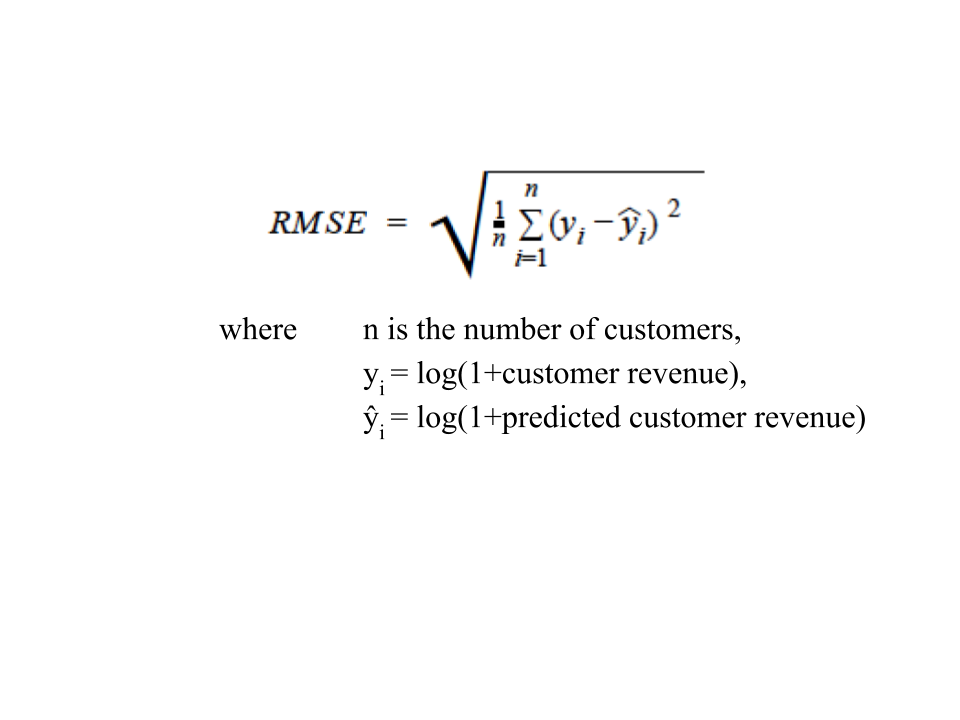
Performance of our proposed methods will be compared to the state-of-the-art methods using Root-Mean-Square Error (RMSE) which is defined as:
Results: Visit-based Model
For results of the visit based model, we show the rmse using 5 fold cross-validation. We use the rmse results from linear regression, polynomial regression and regression tree to compare our model results (these are shown in blue). We compare two variations of our model, one using random forest and one using decision tree, with each baseline. Our results, (shown in grey and orange) show there is a slight improvement to each baseline when using classification with each baseline.

Results: Customer-based Model
For the results of the customer based model, we also show the rmse using 5 fold cross validation. We compare our results to a Recurrent Neural Network baseline. The right graph shows the different hyperparameters used and their results. The hyperparameters for our proposed method that remembered up to 6 visits, 1 hidden or 2 hidden layers, and 6 hidden units showed the best results. With these hyperparameters, were able to provide a slight improvement to the baseline.
Based on the results, we can conclude combining classification and regression can improve the performance of visit based and customer based models with skewed data.

Reference
Competition Website: https://www.kaggle.com/c/ga-customer-revenue-prediction/
- Li, Yanghao et al. “Online Human Action Detection using Joint Classification-Regression Recurrent Neural Networks.” ECCV (2016). https://arxiv.org/abs/1604.05633
- Lathuilière, Stéphane et al. “A Comprehensive Analysis of Deep Regression.” CoRR abs/1803.08450 (2018): n. pag. https://arxiv.org/pdf/1803.08450.pdf
- Cooper, Robin, et al. “Profit priorities from activity-based costing.” Harvard business review 69.3 (1991): 130-135.
- Flach, Peter. (2012). Machine Learning The Art and Science of Algorithms that Make Sense of Data. Cambridge, United Kingdom: Cambridge University Press.
Acknowledgements
We would like to thank the Professor for providing a great course in Machine Learning and we are thankful for the opportunity to complete a challenging project together.